
Spot dispersion or Palladium products have proven successful this year. The payoff is not totally straightforward and the risks associated with that product even less so, let’s take a look.
Payoff description
The payoff is usually written on a basket of stocks (typically 20) 𝑆1,𝑆2,… 𝑆𝑁 and is defined as:
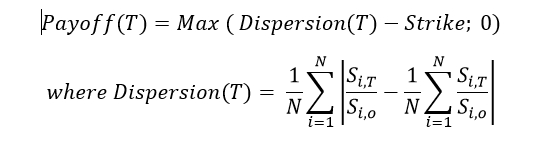
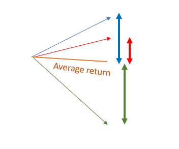
Consequently, dispersion is the average final distance of individual stock returns to the average stock return. Graphically, and in the case of three stocks, the dispersion is the average of the three distances to the average return.
The final payoff is a call on that dispersion. It is important to distinguish that there are two layers of complexity of that payoff:
1. the dispersion itself; and
2. the call on that dispersion.
The maturity of those products is typically two years and the strike can vary between 20% and 40%, so the premium is low, typically in the region of two to five percent. Those warrants can also be packaged into capital-protected notes which are then made of a zero coupon bond and a call on dispersion.
Raison d’être
This product is market neutral and expresses the view that some stocks will do well and some will not, making the final dispersion large. For that reason, it is common to choose a well-diversified basket or to pick stocks that are sensitive to opposite risk factors (growth versus value / US versus Europe / new economy versus old economy etc).
Good backtesting is a key marketing element of those products. If the investment decision is based on that backtesting, then ensuring its stability and robustness should be the investor’s first step. Main questions should be:
- How sensitive is backtesting to maturity: does removing or adding three months change the backtested results dramatically?
- How sensitive is backtesting to the presence of some specific stocks: does removing one or two stocks change the backtested results dramatically?
To illustrate that phenomenon, let us take the example below.
18-month maturity
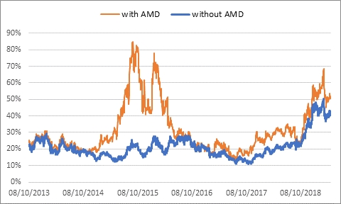
Basket 1: 16 stocks : 3M, AMD, Apple, ASML, Astrazeneca, BP, Facebook, Intesa Sanpaolo, Microsoft, Nestlé, Orange, Pfizer, Rio Tinto, Roche, SAP, Veolia.
Basket 2: 15 stocks: Same as Basket 1 but without AMD.
Plotting the backtesting of the dispersion of those two baskets shows you that the presence of AMD is key in the performance, and that specific backtesting is not very robust to the removal to that specific stock.
Risks at inception
In order to develop some understanding about the risks and the hedging of that product, let us take the simple case where there are only two stocks. In that case, the dispersion formula boils down to:
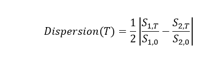
It looks like half a straddle strike zero on . If 𝑆1 and 𝑆2 are lognormal then X will not be lognormal - nevertheless we are going to make that assumption that X is still lognormal with volatility 𝜎𝑋, only to get some intuition of what drives dispersion and what the associated risks are.
Assuming zero interest rates and zero trend, and using the well-known proxy for the price of straddle in Black-Scholes, we have for the expected value of 𝐷𝑖𝑠𝑝𝑒𝑟𝑠𝑖𝑜𝑛(𝑇):
Assuming both 𝑆1 and 𝑆2 have the same volatility 𝜎 and the correlation coefficient between their returns is 𝜌, we have:
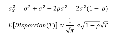
That simple formula allows us to draw important conclusions.
1. The initial delta is null
The initial delta is (almost) null. That was also obvious from the initial payout description, if all stocks are going up or down, the dispersion is unchanged. The initial delta comes only from the skew of the components and other secondary effects.
2. Calls on dispersion are usually very out-of-the-money
Numerically, the formula above gives for reasonable values like 𝜎=30% and 𝜌=60%, 𝐸[𝐷𝑖𝑠𝑝𝑒𝑟𝑠𝑖𝑜𝑛(𝑇)]=15%. Usual palladiums having strikes usually higher than 25%, it shows how out of the money those warrants usually are.
3. The driver of 𝐷𝑖𝑠𝑝𝑒𝑟𝑠𝑖𝑜𝑛(𝑇) is volatility rather than correlation
It is common to hear than exotic desks push those dispersion warrants to hedge their correlation exposure. Indeed it is clear from our proxy result that the higher 𝜌, the lower 𝐷𝑖𝑠𝑝𝑒𝑟𝑠𝑖𝑜𝑛 is.
So exotics traders buy back some correlation risk at inception when selling those warrants, but the main driver of dispersion is volatility. To assess that, let us check what it takes either volatility 𝜎 or correlation 𝜌 to have Dispersion increase by 10%
As dispersion is linear in volatility, if it goes up by 10%, this is equivalent to volatility going up by 10%, so from 30% to 33%. A relative increase of 20%, would mean an increase of volatility from 30% to 36%. Those volatility moves are very possible those days.
For dispersion to go up by 10% only because of correlation, one needs (calling the new correlation 𝜌′):
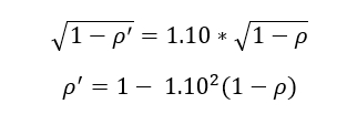
With 𝜌=60%, we have 𝜌′=51.60%.
To increase dispersion by 20%, correlation must go to 𝜌′=1− 1.202(1−𝜌) = 42.40%. Such correlation moves (from 60% to 42.40%) are less likely.
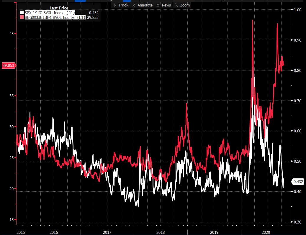
To compare those two moves, you can look at how the one-year implied correlation on SPX stocks moved over the last five years (white line below - mostly contained in a 10% wide range) and, comparatively, how the one-year volatility of the largest cap (Apple) moved over that same period (red line below - 20 vol points range).
(Source Bloomberg)
4. Calls on dispersion are very model-dependent
The dispersion element is dependent on volatility and correlation. An out-of-the-money call on that dispersion will then heavily depend on volatility of volatility and volatility of correlation (and on the correlation between volatility and correlation). As we all know, the value of an out-of-the-money call option is 100% made of time value. In the case of a call on Dispersion, those risks are mainly non-vanilla. If volatility goes up, the expected dispersion will increase (see our proxy formula), so the call on dispersion will become more in-the-money, making it longer volatility: clearly when selling the call on dispersion, exotics traders are short volga (gamma on volatility).
On the contrary, by selling that option, traders are initially long correlation. As correlation goes up, the expected dispersion decreases (see our proxy formula), making the call more out-of-the-money, so the correlation exposure decreases. In other words, exotics traders are also short gamma on the correlation.
Those two elements imply that a model with stochastic volatility and stochastic correlation is necessary to correctly value them.
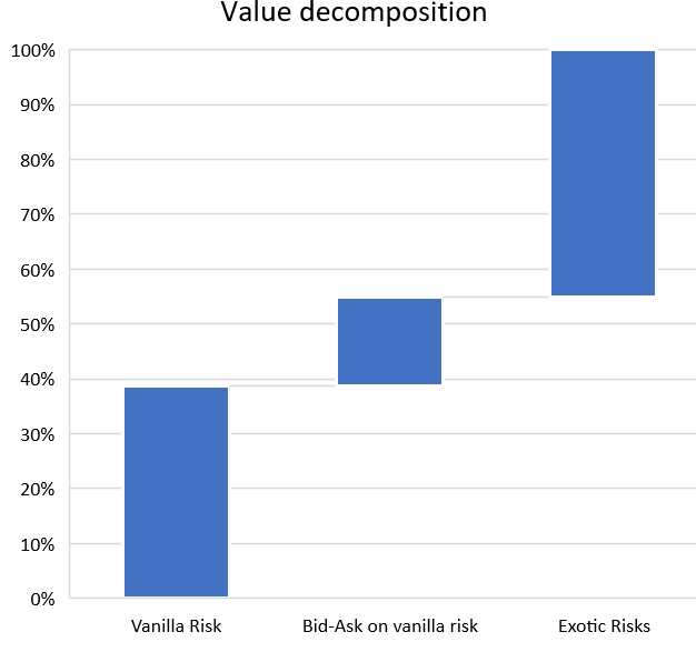
If we were to quantify which elements make the value of a call on dispersion, it would probably look like the below:
5. Dispersion brings tail risk
The initial delta is almost zero. Nevertheless, the trader is short jumps (up or down). Indeed if a stock jumps to default or if one stock is taken over, the value of the dispersion will increase greatly. This is a non-negligible risk: at inception, if one out of the N stocks jumps by J, the impact on the dispersion will be (I assume J positive for simplicity):
(The average return is 𝐽𝑁 , (N-1) stocks have not moved, and 1 stock has moved by J.)
The above formula shows that tail risk decreases with the size N of the basket. To mitigate that risk, those dispersions warrants are usually offered of baskets of more than 15 stocks.
Risks when the trade is alive
As we saw before at inception, main risks are volatility, correlation (they drive the forward), and volatility of volatility and volatility of correlation (which drive the volatility of that dispersion)
As with any option the risks reach their maximum where the option is at-the-money, so in the case of a 25% strike call, when 𝐷𝑖𝑠𝑝𝑒𝑟𝑠𝑖𝑜𝑛(𝑡)≈25%.
This is when the option (on dispersion) starts to have delta (on dispersion). So as an investor you want the dispersion to keep increasing: in other words, you want the outperformers to continue outperforming and the underperformers to keep underperforming. So the situation is quite different from the beginning (when as an investor, you just wanted some stocks to go up and some others to go down). Once dispersion has kicked in the investor becomes long the outperformers and short the underperformers. In that sense, a call on dispersion is a momentum trade. And on the opposite side, the exotic trader is short momentum.
Please note that at this point the correlation risk is not homogeneous anymore, the investor wants outperformers to move together, the underperformers to move together, and the outperformers and underperformers to further diverge. Those are nasty dynamics for the traders as they are now short correlation on stocks that move the most together and long correlation on the stocks that diverge! That is the translation of the short gamma on correlation we mentioned before.
To illustrate that phenomenon, let us take the example of a call on dispersion strike 44% with initial fixing on 1 January 2020, on four stocks (Facebook, Microsoft, Exxon and Schlumberger).
As of the time of writing (20 October 2020), the performances of those stocks are:
- Microsoft: +36%
- Facebook: +27%
- Exxon: -52%
- Schlumberger: -62%
The dispersion is now 44% so the product is at-the-money. The price impact of an increase of five correlation points, per pair is then (point of view of the trader).
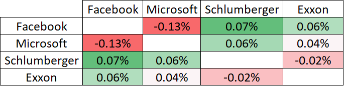
At the beginning, the trader was long on all pairs. But now the trader is short on Facebook/Microsoft correlation and on Schlumberger/Exxon correlation: in other words, they are short on the pairs that correlated the most since the trade started.
As soon as dispersion is far above the strike, the call on dispersion behave likes a long/short portfolio, long the outperformers and short the underperformers. When that situation is reached, the warrant is usually very profitable for the investor.
About Eric Barthe
Eric is currently head of structuring at Anova Partners, based in Zurich, where he drives the firm’s financial engineering efforts.
He started his career as an exotic trader at Goldman Sachs in London. He was there for eight years, trading on the index and single stocks exotic book. After a short interval with the Boston Consulting Group, Eric joined Leonteq as global head of structuring and head of financial engineering.
He was also previously a professor of financial engineering for the MSc International Finance at HEC Paris.
He is a graduate of the Ecole Centrale Paris, HEC and the London School of Economics.